


Introduction
In statistical inference, one of the primary objectives is to estimate an unknown population parameter using sample data. A good estimator should possess desirable properties such as unbiasedness, efficiency, sufficiency, and consistency. Among these, consistency is considered one of the most important large-sample properties because it guarantees that the estimator becomes increasingly accurate as the sample size increases.
A consistent estimator is an estimator that converges to the true value of the population parameter when the sample size tends to infinity. Even if an estimator is biased for small samples, it may still be consistent provided the bias disappears as the sample size grows.
Definition of a Consistent Estimator
An estimator Tn of a parameter  is said to be consistent if, for every positive number
  ,
,

This type of convergence is called convergence in probability. It means that the probability of the estimator differing from the true parameter by more than any fixed positive amount approaches zero as the sample size increases.
Intuitive Meaning
Suppose we repeatedly collect larger and larger random samples from a population and compute an estimator each time. If the estimator is consistent, then its estimates will gradually move closer to the true parameter value. Eventually, for very large samples, the estimator will be extremely close to the actual parameter with very high probability.
Mathematical Condition for Consistency
An estimator Tn is consistent for if

where  denotes convergence in probability.
A commonly used sufficient condition is

When both conditions hold, the estimator is consistent by Chebyshev’s inequality.
Proof Using Chebyshev’s Inequality
Chebyshev’s inequality states that

If

and

then

Hence, Tn is a consistent estimator of .
Examples of Consistent Estimators
1. Sample Mean
Let X1, X2, …, Xn be a random sample from a population having mean  and variance
The sample mean is

Its expectation is

Its variance is
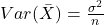
Since

the sample mean is a consistent estimator of the population mean.
2. Sample Proportion
If X follows a Bernoulli distribution with parameter p, then the sample proportion

has

and

Since the variance approaches zero as n increases, the sample proportion is a consistent estimator of p.
3. Sample Variance
The unbiased sample variance

is also a consistent estimator of the population variance
Biased but Consistent Estimator
An estimator does not need to be unbiased to be consistent.
Consider the estimator

Then

which is biased because

However,

Therefore, the estimator is consistent despite being biased for finite samples.
Inconsistent Estimator
Suppose we estimate the population mean using only the first observation:
T=X_1
Then

but
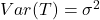
which does not decrease as the sample size increases. Therefore, the estimator does not become more accurate with larger samples and is not consistent.
Properties of a Consistent Estimator
- It converges to the true population parameter as the sample size increases.
- The probability of making a large estimation error approaches zero.
- It is a large-sample property.
- A consistent estimator may be either unbiased or biased.
- If an estimator is unbiased and its variance tends to zero, then it is consistent.
- Consistency ensures reliability for sufficiently large samples.
Difference Between Unbiasedness and Consistency
| Unbiased Estimator | Consistent Estimator |
|---|---|
| Concerned with expectation. | Concerned with convergence as sample size increases. |
| Requires E(T)=. |
Requires T_n . |
| Finite-sample property. | Large-sample property. |
| Variance may remain large. | Variance generally approaches zero. |
| May not be consistent. | May be biased for finite samples. |
Importance of Consistency
- Ensures increasing accuracy as more observations become available.
- Provides reliable parameter estimation in large datasets.
- Forms the theoretical foundation of asymptotic statistical inference.
- Widely used in regression analysis, maximum likelihood estimation, Bayesian methods, and machine learning.
Key Points to Remember
- An estimator is consistent if it converges in probability to the true parameter.
- The formal definition is
 for every .
 - A sufficient condition is and .
- Every unbiased estimator is not necessarily consistent.
- A biased estimator can still be consistent if its bias approaches zero as the sample size increases.
- The sample mean, sample proportion, and sample variance are standard examples of consistent estimators.
 for every
  .
. and
and  .
.Conclusion
Consistency is one of the most fundamental properties of an estimator because it guarantees that the estimator approaches the true population parameter as the amount of available data increases. In practical applications, statisticians often prefer consistent estimators since modern data analysis usually involves large samples. While unbiasedness is valuable for finite samples, consistency provides long-run reliability, making it an essential concept in estimation theory and statistical inference.